architecture

32bit

Introduction

32-bit architectures, sometimes called x86 processors, were introduced in 1979 and were initially the size of 16 bits. However, a processor called 80386 was introduced in 1985, which was of 32 bits size and held a lot of what new processors have built on today. This includes 32-bit general registers, 32-bit data and address buses, a large address space,the introduction of virtual memory, and large changes in the way memory is viewed by a program.

In 1989, the processor 80486 was introduced. This improved upon the 80386 processor and included pipe-lining, floating point registers, on-chip instruction and data caches, and much more. These, however, are out of scope for this introduction.

The next major iteration was the 64-bit processor, which is discussed in a separate lab.

TITLE	DIFFICULTY	TIME	STATUS
Introduction to 64-Bit Architectures	3 Difficulty level 3 of 9	20 Minutes	Completed

Terminology

There are many different terms used to describe 32-bit processors and these are as follows:

• IA-32 – Intel Architecture 32 bit, this is used to describe a 32-bit architecture designed by Intel.
• x86 – This is the instruction set designed by Intel and implemented in the 80386 processor in 1985. This is a family of processors which has now been adopted to describe 32 bit and above.
• i386 – Same as Intel’s IA-32.

These terms and more can be used to describe a computer, file or other such concepts as 32 bits.

Why 32 bits?

A 32-bit architecture is referred to as 32 bits when it can only operate on data up to 32 bits in length; for example, the registers inside the central processing unit (CPU) are of 32 bits in length. However, the data buses and address buses are also of 32 bits in length, which means whenever data is read from memory locations, it can be of a value up to 32 bits in length.

Basic computer organization

There are various aspects which are important to understand. Processors in modern day are increasingly complex; however, there are a few components which are largely similar since the release of processors in the 1940s.

Each computer will have:

• A processor, also referred to as the CPU
• Memory (e.g., RAM) and storage devices (e.g., ROM)
• Input and Output devices

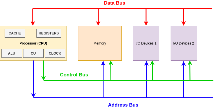
These components are connected using different buses (effectively wires), and these buses are:

• Data Bus – Carries data between the processor and other components; this is a two-way bus
• Address Bus – Carries memory addresses from the processor to other components; this bus goes one way
• Control Bus – Carries control signals for different operations such as read, write, interrupt, clock signals, etc.

The diagram below shows a basic CPU process. The buses on the end of the diagram are going off to other components within the computer.

Processor components

The Control Unit (CU) provides several functions:

• Fetches, decodes and executes instructions – otherwise known as the fetch, decode, execute cycle
• Sends control signals that control hardware components within the CPU
• Transfers data and instructions around the system

The Arithmetic Logic Unit (ALU) has two main functions:

• Performs arithmetic and logical operations (decisions) on data
• Data transferred between primary and secondary storage passes through the ALU, such as memory which is being written to the hard drive after being in RAM.

Registers have a number of functions (more on this later) and they store:

• Address of the next instruction to be executed
• Current instruction being decoded
• Results of calculations from the ALU

Cache

Cache is a small amount of high-speed random access memory (RAM) built directly within the processor. It is used to temporarily hold data and instructions that the processor is likely to reuse. This allows for faster processing, as the processor does not have to wait for the data and instructions to be fetched from the RAM.

Clock

The CPU contains a clock which, along with the CU, is used to coordinate all of the computer’s components. The clock sends out a regular electrical pulse that synchronizes (keeps in time) all the components. This pulse is what transfers and pushes data down the buses. The frequency of the clock is clock speed; the greater the clock speed the more instructions can be executed per second.

Registers

Registers are used to store certain sized data and are designed to be easily accessible by the CPU. There are various registers which historically had specific jobs but have now become general purpose. The two main categories to discuss are general purpose and control registers.

General-purpose registers

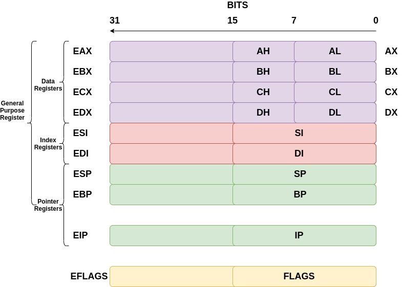
General-purpose registers can be broken down into subcategories of data, pointer, and index registers. The registers discussed below are for a 32-bit architecture; they therefore hold up to 32 bits of data each.

The data registers are EAX, EBX, ECX, and EDX:

• EAX is normally used in any arithmetic operation
• EBX is normally used as a base register to start referring to memory addresses
• ECX is normally the counter register for looping
• EDX is normally the register used for storing data for operations

The pointer registers are EIP, EBP, and ESP:

• EIP is the instruction pointer which holds the memory address of the next instruction to be run
• EBP is the base pointer which holds the memory address of the base of the current stack frame
• ESP is the stack pointer which holds the memory address of the top of the current stack frame

The index registers are ESI and EDI:

• ESI is the source index where the memory location for the start of a string is stored for string operations
• EDI is the destination index where the memory location to store the string after it has been operated on is stored

Control registers

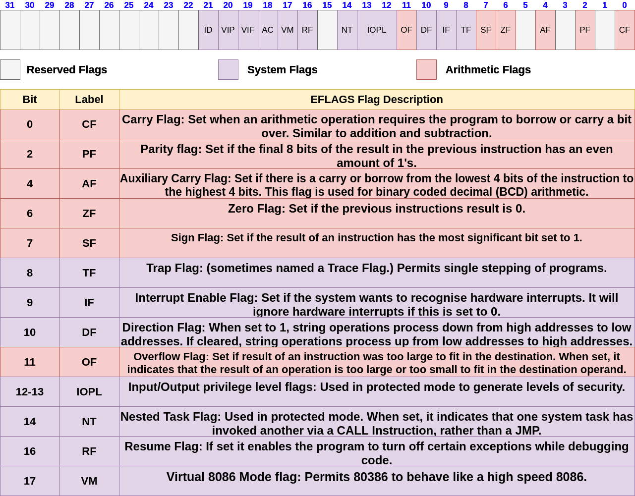
Lots of assembly instructions involve comparing or making mathematical calculations. The eflags register sets either a 0 or a 1 depending on the results of these comparisons or calculations. Once these results are evaluated, the program may need to jump to other branches of code (think if statements for higher level programming languages). There are 32 bits in the eflags register and each bit represents a different evaluation of the previous instruction.

The files allowed to run on this architecture are anything up to 32 bit files; you cannot run a 64 bit file on a 32 bit architecture!

You may have been wondering what the registers for architectures were before 32-bit computers were released. The registers we use are just extended versions of the old registers, hence the ‘e’ at the beginning of each. For some registers, you can reference 16 bits and even 8 bits. For example, to reference the lower 16 bits of the EAX register, we would use AX. The diagram below demonstrates this.

EFLAGS

The eflags register holds a lot of information about the current state of the program. For example, when a compare between two values returns a result of 0, a specific bit is set within the eflags register. There are many different flags inside this register – the main ones are noted in the diagram below.

Protected mode and virtual memory

Within the running of a computer, memory addresses are used to store everything. Files are mapped to locations inside RAM and different sections inside of the file are addressed using memory addresses. These memory addresses can store data or instructions, and the fetch, decode, execute cycle will fetch whatever is at a certain memory address pointed at by either EIP or an instruction, and perform arithmetic tasks on that data.

Earlier, it was stated that the Address Bus is of 32 bits in length, which means that the maximum number of addresses the 32-bit architecture can map to is 2^32 = 4,294,967,296 (which is 4GiB). Therefore, a 32-bit architecture can only map 4GiB of RAM correctly.

Protected mode

With 32-bit processors, protected mode brought a number of new system features to aid in security and memory management. With security it introduced the idea of ring levels, as follows:

• Ring 0 – operating system kernel, system drivers
• Ring 1 – equipment maintenance programs, drivers, programs that work with the ports of the computer I / O
• Ring 2 – database management system, the expansion of the operating system
• Ring 3 – applications, user-run

Ring 3 and ring 0 are generally the most used rings. Ring 3 is limited to a set of instructions which are not considered privileged; therefore, it will not be able to access certain aspects of memory or perform certain tasks. Ring 0, on the other hand, means any instruction is permitted and there are a lot less restrictions on what can be done. The main functionality of the operating system will run in this mode.

With the memory management this will introduce two concepts: virtual memory and paging.

Virtual memory

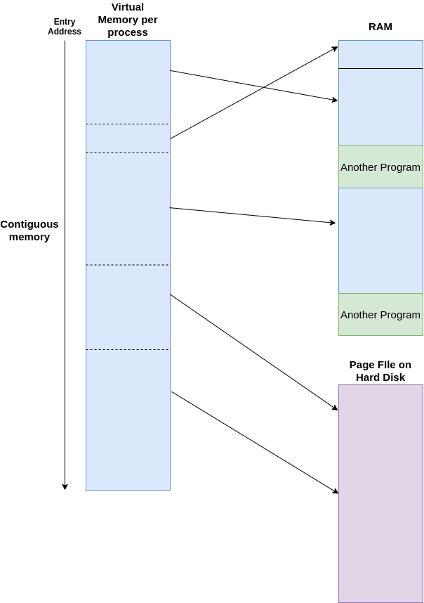
Using a combination of hardware and software, the operating system maps memory addresses used by a program, called virtual addresses, into physical addresses in computer memory (RAM). Main storage, as seen by a process or task, appears as a contiguous address space or collection of contiguous segments. Therefore, a program will get loaded into a typical memory address of 0x40000000 for Linux, for example, but its actual physical address is hidden by the operating system. The program assumes that it has access to all the contiguous memory it needs from the address 0x40000000, but in reality it is simply is placed in different areas of the physical address. This introduces the concept of paging.

paging

This is where the program will get loaded in small ‘pages’ into RAM, for example, of size 4Kb. This is done to control the space of RAM more effectively. The operating system uses page tables to translate the virtual addresses seen by the application into physical addresses used by the hardware to process instructions. Each entry in the page table holds a flag indicating whether the corresponding page is in real memory or not. If it is in real memory, the page table entry will contain the real memory address at which the page is stored. When a reference is made to a page by the hardware, if the page table entry for the page indicates that it is not currently in RAM, the hardware raises a page fault exception, which means the operating system will then go and load more of the file in memory (another 4Kb).

When the OS realizes there are pages in RAM that are not often used, it can move those pages into the Hard Disk in a file called page file. This will effectively be a slower extension of RAM – not everything can be placed into the page file, such as most kernel functionality, but for programs that are running in the background and are laying dormant it might place them in the page file.

These two concepts are complex, but this is an introduction into what aspects 32-bit architectures introduce. The image below shows how virtual memory is shown to a program according to the program running; the memory addresses it can access are contiguous, whereas from this image it shows different sections are interleaved with other programs in RAM.

64bit

Introduction

64-bit architectures are an iteration of the 32-bit processors which were introduced in 1985. The first release of the 64-bit version of the 32-bit architecture, x86, was in 1999; it contained a compatibility mode, 64-bit mode, and a new four-level paging mode. Furthermore, it expanded on the general purpose registers and added more usable registers for the program.

Terminology

There are many different terms used to describe 64-bit processors and these are described here:

• Intel 64 – Intel Architecture 64 bit, this is used to describe a 64-bit architecture designed by Intel
• x86_64 – This is the instruction set that is an extension of the x86 architecture
• x64 – Same as x86_64
• AMD64 – Used to describe AMD’s 64-bit instruction set.

Why 64 bits?

A 64-bit architecture is referred to as 64 bits when it can operate on data up to 64 bits long; for example, the registers inside the central processing unit (CPU) are of 64 bits in length. However, the data buses and address buses are also of 64 bits in length, which means whenever data is read from memory locations, it can be of a value up to 64 bits in length theoretically.

For information on how a processor is organised, it is recommended you complete the lab listed below first.

Introduction to 32-Bit Architectures

[Completed 17/02/2023Practical Lab

3

40 Points20 Minutes

In this lab, we will be examining what 32-bit architectures are, what sort of files can run on them, and what is happening behind the scenes when they’re interacting with your operating system. 

View Lab](https://arcticwolf.immersivelabs.online/labs/introduction-to-32-bit-architectures-6430e3df-a4fd-4798-b5da-32624030f58b/)

Compatibility Mode

The 64-bit architecture introduced a compatibility mode, which meant that files that were compiled for 16-bit and 32-bit operating systems could still run unmodified, and could effectively run alongside the 64-bit programs on a 64-bit operating system. This is because inside the instruction set x86_64, 16-bit and 32-bit instructions are also supported! Therefore, you can use the smaller size registers for any operations. The older executables can run with little or no performance penalty, while newer or modified applications can take advantage of new features of the processor design to achieve performance improvements.

Registers

Registers are used to store certain sized data and are designed to be easily accessible by the CPU. There are various registers which historically had specific jobs but have now become general purpose. The two main categories to discuss are general purpose and control registers.

General purpose registers

Inside general purpose registers, it can be broken down into sub categories: data, pointer and index registers. The registers discussed below are for a 64-bit architecture, and therefore hold up to 64 bits of data inside each.

The data registers are as follows:

• RAX is normally used in any arithmetic operation.
• RBX is normally used as a base register to start referring to memory addresses.
• RCX is normally the counter registers for looping.
• RDX is normally the register used for storing data for operations.
• R8-R15 registers are normally used to hold certain data for any operations.

The pointer registers are RIP, RBP and RSP.

• RIP is the instruction pointer which holds the memory address of the next instruction to be run.
• RBP is the base pointer which holds the memory address of the base of the current stack frame. If there are certain optimisations made by the assembler, RBP becomes another general purpose register!
• RSP is the stack pointer which holds the memory address of the top of the current stack frame.

The index registers are RSI and RDI.

• RSI is the source index where the memory location for the start of a string is stored for string operations.
• RDI is the destination index where the memory location to store the string after it has been operated on is stored.

You may have been wondering about the registers for architectures before 64 bit computers were released. The registers we use are just further ‘extended’ versions of the older 32-bit registers, such as EAX. The ‘R’ stands for register and is a way to know a register is 64 bits. For some registers, you can reference 32 bits, 16 bits and even 8 bits. For example, if you wanted to reference the lower 32 bits of the R15 register, you would use R15d. The diagram below demonstrates this.

Control registers

Lots of assembly instructions involve comparing or making mathematical calculations. There is a register called the rflags register which sets either a 0 or a 1 depending on the results of comparisons or calculations. The purpose of this register is once these results are evaluated, the program may need to jump to other branches of code (similar to if statements for higher level programming languages). There are 64 bits in the rflags register and each bit represents a different evaluation of the previous instruction.

RFLAGS

The rflags register holds a lot of information about the current state of the program. For example, when a comparison between two values returns a result of 0 (akin to a ‘false’ if statement), then a specific bit is set within the rflags register. There are many different flags inside this register – the main ones are noted in the diagram below. Everything from bit 32-63 is reserved and set to 0.

Bus sizes

Inside a computer, there are many buses which are used to transfer different information around the circuits. These are and not limited to the data bus, address bus and control bus. The comparison between 32-bit and 64-bit processors are as follows:

Note:

In principle, a 64-bit processor can address 16 EiBs (2^64 = 18,446,744,073,709,551,616 bytes, or about 18.4 exabytes) of memory. However, processors in practice do not support a full 64-bit virtual or physical address space. Instead, they generally use 48 bits, which is 2^48 281,474,976,710,656 bytes, or 281.5 terabytes of memory.

Four Level Paging

Paging was first discussed at a basic level in the Introduction to 32 bit architecture lab.

Four level paging was introduced in 64-bit architectures to better process memory addresses. From a virtual memory address (the memory address shown to the program), the operating system can use a set of page tables to find the underlying physical addresses which are associated with the virtual address.

The diagram below describes this process:

Breaking down the image above, there are several aspects to consider. Firstly, the virtual address can be broken down into different sections which act as an offset or index into the respective tables. For example, the above diagram shows bits 21–29 are the Page-Directory Offset which, once added to the base address given from the previous table (Page-Directory Pointer Table), will give the base address for the Page Table which will know where the base address of the Physical page is in RAM.

In the 32-bit architecture lab we said that normally a page size is 4Kb, so each virtual address will map to a certain Physical Address range and the final 12 bits in the virtual address will be the actual offset inside that 4Kb space in RAM.

The computer will always know where the Page-Map Level 4 Base Address is and uses the offsets and the tables to effectively walk from each table to the next until a physical address is retrieved.

Some abbreviated terms from the diagram are explained below:

• PML4E – Page-Map Level 4 Entry, this is the entry inside the Page-Map-Level 4 which gives the base address of the relevant Page-Directory Pointer Table.

• PDPE – Page-Directory Pointer Entry, this is the entry inside the Page-Directory Pointer Table which gives the base address of the relevant Page-Directory Table.

• PDE – Page-Directory Entry, this is the entry inside the Page-Directory Table which gives the base address of the relevant Page Table.

• PTE – Page Table Entry, this is the entry inside the Page Table which gives the base address of the relevant Page residing in physical memory.

Memory

Memory hierarchy

In the context of computer architecture, memory is a physical device capable of storing information. When you think about memory, you might think of your hard drive. While this is technically correct, a hard drive is just one of the many devices that make up the memory hierarchy of a modern computer.

The hierarchy represents a trade off between speed of access and storage space. For example, your desktop can typically access information stored in a register in under one nanosecond (0.000000001 seconds), but in general, each register will only be able to store a maximum of 64 bits at a time. Contrastingly, hard disks can have upwards of one terabyte (TB) of space, but can take around 10 milliseconds (0.01 seconds) to access.

Memory addressing

What does it mean to ‘access’ memory? In general, memories allow two basic operations: read and write. As the names suggest, the write function allows information to be stored in memory, and the read function extracts said information to be manipulated. However, there needs to be a way of specifying where this information is stored and extracted from. That’s where memory addressing comes in.

Each piece of information is assigned a unique number (known as an address) in the memory. By passing this value as an argument, we can manipulate the value stored there and overwrite it if it’s no longer required.

One technique, called memory-indirect addressing, allows passing the value stored in another part of memory as a variable. This might look something like:

MEM[ MEM [10] ] <- r1

MEM is our DRAM and r1 is a register. We are telling the computer to use the value stored in memory address 10 as the new address to write the content of r1 into. Direct addressing, where a value for the address is given, would look like:

MEM[ 10 ] <- r1

Here, we are telling the computer to set the value in address 10 to what’s stored in r1. This is quicker than memory-indirect, as we do not need to fetch data from another part of memory, but the address cannot be dynamically computed. Each addressing mode comes with a trade off between speed of access and range of memory addresses that can be specified for flexibility.

Data vs instructions

Information in the general sense is stored as described above, but there are two specific types that we’re interested in. Data is information operated on by the CPU in calculations (integers, characters, etc.), whereas instructions specify what must be done with the data (ADD, DIV, etc.).

The diagram below shows a high level version of how data and instructions interact with the CPU.

Depending on the CPU’s architecture, each instruction is encoded in some way as control information; the actual binary signals that perform the logical operations at the lowest level of a computer’s architecture. As such, the amount of memory required to store these instructions is massive. The solution to this is to use op-codes – unique encodings assigned to each instruction – that when passed through a decoding module, result in the desired control information. Decoding is done in a variety of ways, including with combinatorial, lookup, and DMUX (demultiplexer) based methods.

The Heap

Every computer needs memory to store data. The running memory of a computer is stored in RAM; however, computer programs also need memory to run. There are two main types of memory for programs: the heap and stack. This lab discusses what the heap is at a high level, and as you analyse programs within debuggers and disassemblers, your practical knowledge of the heap will inevitably increase!

Heap is a memory region given to every program. Unlike the stack, heap memory can be dynamically allocated, meaning the program can allocate and de-allocate memory while the program is running. Heap memory is globally accessible, so it can be accessed and modified from anywhere within a program and is not localised to the function where it is allocated, just like local variables are for the stack. This is accomplished using pointers (memory addresses) to reference dynamically allocated memory, which in turn leads to a small degradation in performance as compared to using local variables.

The heap grows from a low address to a higher address (as you would think is normal); it grows towards the stack. The stack grows from a high address to a lower address and also grows towards the stack. Memory is structured like this due to memory constraints when computers were first being developed. The stack and heap were placed in the same region to keep memory management low and cheap. Below is a diagram which shows this:

As you can see from the diagram above, the executable already knows the size of the memory that will be needed to fulfil the program’s tasks, and the OS loader will therefore create enough space for the program in RAM. Let’s break down what the heap is explicitly used for and then what the heap looks like.

How to use the heap

The heap can be used through C with two functions: malloc and free.

Malloc takes a single parameter, which is the size of the requested memory in bytes. It returns a pointer to the allocated memory. If the allocation fails, it returns NULL.

Free takes the pointer returned by malloc and de-allocates the memory. No indication of success or failure is returned. This can be any part of the heap that gets freed and can eventually lead to fragmentation (more on this later).

The following code does the same job using dynamic memory allocation:

int *pointer;
pointer = malloc(10 * sizeof(int));

When the array is no longer needed, the memory can be de-allocated thus:

free(pointer);
pointer = NULL;

Assigning NULL to the pointer is good practice; it means an error will be generated if the pointer is erroneously used after the memory has been freed.

The amount of heap space allocated by malloc is normally slightly larger than the requested size. The additional space is used to hold the size of the allocation and is used by free later when called.

When allocating memory on the heap, there is a restriction in that the memory block has to be contiguous and large enough to satisfy the request. This means the memory manager that carries out the allocation operation must scan the heap until it finds a memory block large enough that is contiguous.

There is only one restriction on the memory that is allocated to the program from the heap: it must form a contiguous block large enough to satisfy the request with a single chunk of memory. When that memory is freed, the chunk will be de-allocated and put into a ‘bin’, which can be reallocated in the future. The heap’s complexity means that managing memory with a heap is slower and less efficient than doing so with a stack.

Below is a diagram of the structure of a chunk of allocated memory on the heap.

Let’s break down the image above:

• Memory pointer is the pointer returned to the program after executing malloc; it is the location where the user data will go
• A – Allocated arena. If this bit is 0, the chunk comes from the main heap of the application. If this bit is 1, the chunk comes from mmapd memory and the location of the heap can be computed from the chunk’s address.
• M – Mmapd chunk. This bit is set if this chunk was allocated with a single call to mmap and is not part of a heap at all.
• P – Previous chunk is in use. If set, the previous chunk is still being used by the application.
• Chunk pointer is the base memory address of the chunk.

Once a chunk has been allocated, it can be de-allocated with free; this will change the chunk’s data to look like the image below:

The main difference between a freed chunk and an allocated chunk is that the data is zeroed out. The flag M is also taken away because it is no longer mapped to the application. The chunk is updated to a list of freed different memory bins which are organised in certain sizes (these can be reallocated later). Sometimes these chunks of memory are freed as well as their contiguous chunk, meaning that a larger chunk of memory could fill those two smaller chunks if there was memory of that size being requested.

Memory Fragmentation

Memory fragmentation

Memory fragmentation occurs when contiguous blocks of memory are used – the blocks can be of different sizes. Then, parts of the memory are de-allocated. If a new part of memory was to be allocated and it was of a smaller size than the space previously de-allocated, it would cause spaces inside the memory structure. The diagram below explains this:

Heap Pros v Cons

There are several advantages and drawbacks to the heap:

Pros

• Variables can be accessed globally
• No limit on memory size
• Variables can be resized using realloc

Cons

• Slower access

• No guaranteed efficient use of space, memory may become fragmented over time as blocks of memory are allocated, then freed

• The programmer must manage memory (you’re in charge of allocating and freeing variables)

What is the stack?

Stack is a form of memory that programs use to store local data to a function. It acts as a first-in-last-out buffer and will always be contiguous. Programs use the stack for a few different reasons, though it is important to note that the program has full control over what goes on its stack frames.

The stack is looked after by two registers local to the CPU: the stack pointer and base pointer. These are ESP and EBP for 32-bit architectures, and RSP and RBP for 64-bit architectures. (More on how they track the stack later.)

When the stack was initially introduced memory was limited, which meant the two forms of memory for a program, stack and heap, were placed in a similar region to reserve space across the RAM. This means the heap grows from a lower address towards a higher address, whereas the stack grows from a higher address to a lower address. This is shown with the sections of an executable in the diagram below:

When the executable is compiled, a lot of information about how much memory will be needed is stored. Therefore, when the executable is loaded, the OS already knows the size of the memory that will be needed to fulfil the programs tasks. Let’s break down what the stack is used for explicitly and then examine the appearance of the stack frames.

How to use the stack

The stack is used for local variables relating to a function. The code below will therefore create several different variables on the stack.

Declaring local variables

int Main()
{
int i;
int number = 20;
int *i;
}

The code above declares a number of integer variables on the stack. On a 32-bit system, this will be three sets of 32-bit values. These will all be declared in the main() stack frame and will only be accessible while the main() function of the program has code executing. The image below describes how these will look on the stack:

As stated before, the stack is a first-in-last-out buffer, so let’s break down the image above to see what is actually happening. The source code shows:

int i;
int number = 20;
int *i;

Recall that the stack grows from a high address to a lower address. These variables are local to this function, which means they are declared and manipulated on the stack. Generally, the program will run a set of instructions at the beginning of a function called the function prologue, which will set up the stack for the local variables inside the function. For the function above, the prologue could look something like this:

mov ebp, esp

sub esp, 0xC

EBP is the base pointer of the current stack frame and will therefore hold the memory address of the first element of the current stack frame. ESP is the memory address of the top of the stack. Therefore, this is changing EBP to point to the top of the current stack frame in order to make a new stack frame for this function.

ESP will always point to the top of the stack, so in the function prologue, a value will get subtracted against ESP, which will effectively grow the stack towards a lower memory address. This will create a new stack frame. Once this is done, the program knows that to reference any part on the stack, it can use either EBP - a value or ESP + a value. The diagram below illustrates this:

Accessing variables

The image above shows several ways to reference variables from the EBP or ESP register. This will be done inside the assembly of the program.

EBP - 4 for example will reference the i variable. ESP + 8 will also reference the same variable!

Function calls

Function calls utilise the stack in 32-bit architectures, and under certain circumstances, they do in 64-bit architectures as well. This will describe how the stack is used for function calling.

• When a function is called, a new stack frame is created
• • Arguments to the functions are placed on the stack
    • Current frame pointer (EBP register which points to the base of the current stack) and return address are placed on the stack
    • Memory for local variables is allocated with the function prologue
    • Stack pointer is adjusted with the function prologue
• When a function returns, the top stack frame is removed
• • Old frame pointer and return address are popped off the stack and placed in EBP and EIP (instruction pointer) respectively
    • Stack pointer is adjusted within the function epilogue

The assembly instruction to place a value on the stack is PUSH which automatically places a value on the stack and decrements ESP (subtracts 4 bytes to the memory address inside ESP).

The assembly instruction to take a value off the stack is POP which automatically takes a value off the stack and increments ESP (adds 4 bytes to the memory address inside ESP).

Below is a diagram which shows code and how it interacts with the stack frames. This is effectively a snapshot of the stack if the return is 0; inside the func() function was the next instruction to execute.

Stack pros and cons

There are several pros and cons to using the stack:

Pros

• Access to the stack variables is much faster than other memory structure
• Programmer doesn’t have to explicitly de-allocate variables
• The space is managed efficiently by CPU, so memory will not become fragmented

Cons

• Local variables only
• Limit on stack size (OS-dependent)
• Variables cannot be resized

Security issues

There are issues relating to the stack which can cause major security issues within memory and even lead to full compromises of applications:

• There is no default initialisation for stack variables
• • Reading uninitialised local variables, memory content can be read that is used in earlier function calls
• There is only finite stack space
• • A function call may fail because there is no more stack memory
• The stack mixes program data and control data

• • Overrunning buffers on the stack, the return addresses can be corrupted as the return address on the stack gets put into EIP the instruction pointer register so code can be redirected

Linux

The Linux operating system (OS) has been around for a long time. A hugely popular OS, it is used by server companies, security professionals, developers and more. It can be very lightweight and is similar to the Windows OS in many respects. In this lab, there will be discussion on the architecture, the different modes of execution, and the address space. Further learning about the Linux OS will be done in the Linux assembly series.

Linux architecture

The Linux architecture is broken up into two modes: Kernel mode and User mode.

Kernel mode is reserved for the operating system functionality and is a mode that gives less restrictions to accessing memory and other such important hardware resources.

User mode is for user applications; these applications require a lot more control, which will be managed by the operating system. Therefore, if a user application wants to access memory or privileged resources, it will have to use API functions exposed by the kernel in order to do so.

The kernel offers a set of APIs that applications use. These APIS aregenerally referred to as System Callsor syscalls. They are different from regular library APIs because they are the boundary at which the execution mode switches from User mode to Kernel mode. These system calls rarely change between updates in order to provide compatibility across different Linux versions.

The image below explains, at a high level, the Linux architecture, and shows how the user applications go through the shared libraries in order to access Linux kernel functionality:

Memory Addressing

The address space in Linux operating systems takes advantage of the Protected mode that 32-bit processors have introduced. Virtual memory addressing is used to effectively trick the program into thinking it has contiguous memory blocks, when in reality sections of the program can be scattered across RAM. The kernel will map virtual memory addresses to physical addresses.

However, the user applications in 32-bit processors can see 2^32 addresses, which is 4GiB.Many of these memory addresses are reserved for kernel functionality. There is a lot more addressable space when using 64-bit processors. The diagram below shows 32-bit addressing and where the kernel and user application code can be mapped:

Processes

A process in Linux is the entity which represents the basic unit of work to be implemented in a system. This means that once an executable is created and executed, it becomes a process. The process has a lot of different aspects to it, mainly a large set of information used by the OS to understand what the process is. It also has a process life cycle which is tracked by the OS.

Process lifecycle

When a process executes, it passes through different states. These stages may vary in different operating systems, but generally the states are the same:

• Start – The initial state when a process is first created
• Ready – Process is waiting to be run by the processor
• Running – Process is currently running on the processor
• Waiting – Process is in a waiting state (if, for example, it is waiting for user input or a resource to be freed)
• Terminated – A process has been finished by the OS

The image below shows the lifecycle of a process:

All the process information is contained in a structure called the process control block (PCB). This information is needed to keep track of the process and contains several pieces of information:

• Process state – Where in the life cycle the process is
• Process privileges
• Process ID
• Pointer – This points to the parent process
• Program counter – Pointer to the next address to be executed
• CPU registers – where data needs to be stored
• CPU scheduling information
• Memory management information
• Accounting information
• Input/output status information

The PCB will last while the process is running; once terminated, the PCB will also be deleted.

Linux Shells

The shell provides user applications and users a way to communicate with the kernel. The most popular shell is bash, and we recommend that you learn about this. A user can run commands in the command line interface (CLI), and the kernel will fulfil the command requirement if needed to do so. Most commands are simply wrappers around system calls which are used to switch the context of User mode to Kernel mode. The shell can be used as a gateway into the kernel where the majority of commands will go through this process.

Scheduling

All operating systems have to schedule tasks. These tasks are processes to be executed on the CPU; they cannot occur simultaneously because there is a limited amount of cores. Also, the CPU can’t run a full process from beginning to end and then simply start another. If this was the case, then the computer would not be able to display everything, check permissions, fetch memory, and do all the other tasks a CPU needs to do.

Linux inherits the Unix view of a process – as a program in execution. A process must contend with other processes for shared system resources, such as memory, which holds instructions and data, at least one processor to execute instructions, and I/O devices to interact with the user (for example, keyboard, mouse and screen).

Process scheduling is how the OS assigns tasks defined by processes to processors. A process has one or more threads of execution, which are sequences of machine-level instructions. To schedule a process is to schedule one of its threads on a processor.

Linux uses the completely fair scheduler (CFS), which can be broken down into a few steps at a high level. In practice, a lot of privileged tasks will come in and get execution time over user applications.

When the scheduler is invoked to run a new process…

• The process with the least spent execution time is sent for execution from the queue.

• • If the process simply completes execution, it is removed from the system and scheduler.

• If the process reaches its maximum execution time or is otherwise interrupted, it is reinserted into the scheduler based on its new spent execution time.

• A new task will be taken from the queue and this process is repeated.

Linux ELF

The Executable and Linkable Format is a common standard file format for Linux executable files, object code, shared libraries and core dumps. Within a cyber security context, ELF binaries are a common artefact to reverse engineer; they are also used to develop exploit code and malware and other forensic investigations.

When attempting to reverse engineer an unknown ELF binary, there are tools we can use to expose important information about the structure of the executable. Tools such as objdump and readelf let us see the architecture a binary was written for, and the location of program and section headers. They also let us check to any library was used and the entry point of an executable.

ELF specs

Introduction

The Executable and Linkable Format, ELF, is widely used for executable files, relocatable object files, shared libraries and core dumps. It is the standard binary file format for Unix systems as of x86 processors. There are two components to an ELF executable: the ELF header and file data. The file data can be broken down into subcomponents, which are program header and/or section header, and the actual data. This will be described later in the lab.

Below is an illustration of the structure of an ELF executable:

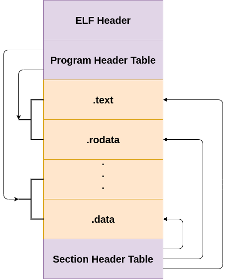
ELF Header

The ELF header is the first component to the ELF executable. It starts with the sequence 0x7f454c46which in ASCII is .ELF. These are the magic bytes for the file. After the magic bytes, the file header contains a number of different pieces of data which helps the loader within a Unix system understand what sort of information is stored within the file. Below is the header definition of an ELF executable in /usr/include/elf.h.

At the start of each ELF file is an ELF header that describes the file contents. The first four bytes is a ‘magic’ number containing 0x7f,’E’,’L’,’F’ that the system uses to ensure it is an ELF file.

Other entries in this header include whether the file is 32 bit or 64 bit and the endianness of the numbers. Big endian means that the highest-value byte is placed first, followed by the lowest-value byte; little endian means the lowest-value byte is placed first, followed by the highest-value byte. For example, a value of 0xABCD would be stored as 0xAB, 0xCD as a big endian and 0xCD, 0xAB as a little endian.

The ELF header also contains fields for the target operating system, the program code type, and the processor instruction set the program is compiled for. This is important, as ELF files are used on a variety of different platforms with different processors.

Program header

The program header provides information that’s used to create the process image, such as dynamic linking.

Section header

A program resident in computer memory is split into different sections, and these sections are represented in an ELF file by section headers.

The first header field is the name of the section as it should appear in memory. Program code is usually placed in a section called ‘.text’.

Another section, ‘.data’, is used to store global data variables that are accessible from anywhere within a program. It is also used to store static local variables that behave like normal local variables and have visibility limited to their function (but they retain their values between multiple calls to that function).

Programs also use symbol tables that link names of functions, such as the C function called ‘main’, to their locations within memory. These symbol tables are represented in an ELF file by section headers.

ELF Header Struct

// 32 Bit Header Executabletypedef struct
{
unsigned char e_ident[EI_NIDENT]; /* Magic number and other info /
Elf32_Half e_type; / Object file type /
Elf32_Half e_machine; / Architecture /
Elf32_Word e_version; / Object file version /
Elf32_Addr e_entry; / Entry point virtual address /
Elf32_Off e_phoff; / Program header table file offset /
Elf32_Off e_shoff; / Section header table file offset /
Elf32_Word e_flags; / Processor-specific flags /
Elf32_Half e_ehsize; / ELF header size in bytes /
Elf32_Half e_phentsize; / Program header table entry size /
Elf32_Half e_phnum; / Program header table entry count /
Elf32_Half e_shentsize; / Section header table entry size /
Elf32_Half e_shnum; / Section header table entry count /
Elf32_Half e_shstrndx; / Section header string table index /
} Elf32_Ehdr;// 64 Bit Header Executabletypedef struct
{
unsigned char e_ident[EI_NIDENT]; / Magic number and other info /
Elf64_Half e_type; / Object file type /
Elf64_Half e_machine; / Architecture /
Elf64_Word e_version; / Object file version /
Elf64_Addr e_entry; / Entry point virtual address /
Elf64_Off e_phoff; / Program header table file offset /
Elf64_Off e_shoff; / Section header table file offset /
Elf64_Word e_flags; / Processor-specific flags /
Elf64_Half e_ehsize; / ELF header size in bytes /
Elf64_Half e_phentsize; / Program header table entry size /
Elf64_Half e_phnum; / Program header table entry count /
Elf64_Half e_shentsize; / Section header table entry size /
Elf64_Half e_shnum; / Section header table entry count /
Elf64_Half e_shstrndx; / Section header string table index */
} Elf64_Ehdr;

From the two STRUCTs above, there are few difference between a 64-bit header and 32-bit header. The main difference is that when the e_machine value is looked at, it will indicate x86-64 instead of x86. Below is the header displayed for the /bin/ls executable on Linux.

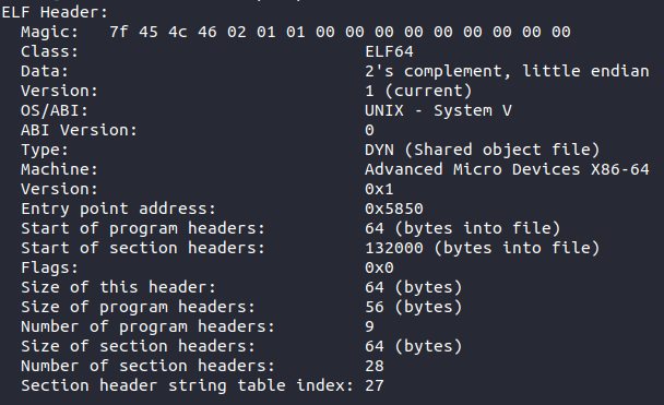
Breaking down the individual parts of the ELF header:

• Type – The type of file, e.g., executable file, shared object, core dump
• Machine – What type of machine this file was compiled for, can be x86-64, ARM etc.
• Version – Either 0 or 1, normally 1
• Entry – Gives the virtual address to the beginning of the executable section of the file
• Program Header Offset – Location of the program header within the executable file
• Section Header Offset – Location of the section header within the executable file
• Flags – No flags are defined, so will be 0
• ELF Header Size – The size of the ELF header in bytes
• Program Header Entry Size – Size of one entry in the reference by the program header – each entry is the same size
• Program Header Number – The number of entries in the program header
• Section Header Entry Size – Size of one entry in the reference by the section header – each entry is the same size
• Section Header Number – Holds the number of entries in the section header
• Section Header String Table Index – Holds the section header table index of the string table entry within the file

Program header

The program header is a part of the ELF executable which describes a segment within the file. A segment is a collection of sections that have the same information for the loader to understand the sort of protections associated to them. For example, the .bss and .data section should not be executable, but the .textsection needs to be, therefore the compiler could group the .text section into one segment and the .bssand .data section into a separate segment. The program header is used by the loader to determine which parts of the file will be placed where and what sort of protections and data are connected to it.

Below are the STRUCT definitions for the program header for both 32 and 64 bit:

Program Header Struct

// 32 Bit Program Headertypedef struct
{
Elf32_Word p_type; /* Segment type /
Elf32_Off p_offset; / Segment file offset /
Elf32_Addr p_vaddr; / Segment virtual address /
Elf32_Addr p_paddr; / Segment physical address /
Elf32_Word p_filesz; / Segment size in file /
Elf32_Word p_memsz; / Segment size in memory /
Elf32_Word p_flags; / Segment flags /
Elf32_Word p_align; / Segment alignment /
} Elf32_Phdr;// 64 Bit Program Headertypedef struct
{
Elf64_Word p_type; / Segment type /
Elf64_Word p_flags; / Segment flags /
Elf64_Off p_offset; / Segment file offset /
Elf64_Addr p_vaddr; / Segment virtual address /
Elf64_Addr p_paddr; / Segment physical address /
Elf64_Xword p_filesz; / Segment size in file /
Elf64_Xword p_memsz; / Segment size in memory /
Elf64_Xword p_align; / Segment alignment */
} Elf64_Phdr;

The important parts of the program header are described here:

• Type – Indicates what kind of segment, the important ones are as follows:
• • PT_NULL – This segment is ignored
    • PT_LOAD – Specifies a loadable segment which will be loaded into memory
    • PT_INTERP – The array element specifies the location and size of a null-terminated pathname for the interpreter
• Offset – Holds the offset from the beginning of the file at which the first byte of the segment resides
• Virtual address – The virtual address of the segment once it is loaded in memory
• Physical address – Same as the virtual address now
• File size – Holds the size of the segment in the file
• Memory size – Holds the size of the segment in memory; this can be different from file size because some sections will contain more data within memory than in the file
• Flags – Shows information about the segment
• • PF_X – An executable segment
    • PF_W – A writable segment
    • PF_R – A readable segment

Generally, a code segment will be executable and readable whereas a data segment will be writable and readable. If these are different, that could be a way to exploit a binary or tell if there is something malicious going on.

Section header

The section header stores information about the sections inside the file. This header never gets loaded into memory; it is purely there for the linker to understand where the sections are so it can sort relocations and other such linker jobs. Below are the structures defining the section headers within /usr/include/elf.h.

Section Header Stuct

// 32 Bit Section Headertypedef struct
{
Elf32_Word sh_name; /* Section name (string tbl index) /
Elf32_Word sh_type; / Section type /
Elf32_Word sh_flags; / Section flags /
Elf32_Addr sh_addr; / Section virtual addr at execution /
Elf32_Off sh_offset; / Section file offset /
Elf32_Word sh_size; / Section size in bytes /
Elf32_Word sh_link; / Link to another section /
Elf32_Word sh_info; / Additional section information /
Elf32_Word sh_addralign; / Section alignment /
Elf32_Word sh_entsize; / Entry size if section holds table /
} Elf32_Shdr;// 64 Bit Section Headertypedef struct
{
Elf64_Word sh_name; / Section name (string tbl index) /
Elf64_Word sh_type; / Section type /
Elf64_Xword sh_flags; / Section flags /
Elf64_Addr sh_addr; / Section virtual addr at execution /
Elf64_Off sh_offset; / Section file offset /
Elf64_Xword sh_size; / Section size in bytes /
Elf64_Word sh_link; / Link to another section /
Elf64_Word sh_info; / Additional section information /
Elf64_Xword sh_addralign; / Section alignment /
Elf64_Xword sh_entsize; / Entry size if section holds table */
} Elf64_Shdr;

The important components of the section header are described below:

• Name – Specifies the name of the section
• Type – Indicates what kind of section; the important ones are:
• • SHT_PROGBITS – This stands for programmable bits, where the programmer has defined what is inside this section
    • SHT_SYMTAB – This section holds a symbol table
    • SHT_STRTAB – This section holds a string table
    • SHT_NOBITS – A section of this type occupies no space in the file
• Flags – Shows information about the section
• • SHF_WRITE – This section contains data that should be writable during process execution
    • SHF_ALLOC – This section occupies memory during process execution
    • SHF_EXECINSTR – This section contains executable machine instructions
• Address – The location of the first byte if this section was to be loaded into memory
• Offset – Holds the byte offset from the beginning of the file to the first byte in the section
• Size – Holds the section’s size in byte

Sections

There are several different sections that are defined by the ELF file format. The most common and useful ones to understand are as follows:

• .text – This section contains the executable code of the program. This is important for malware analysis and reverse engineering

• .bss – This section contains uninitialised data variables; for example, in C when declaring a variable such as this int i;. This is important for malware analysis and reverse engineering.

• .data – This section contains initialised data variables; for example, in C when declaring a variable such as this int i = 0;. This is important for malware analysis and reverse engineering.

• .rodata – This contains only read-only data such as when a const is declared in C. This is important for malware analysis and reverse engineering.

Windows Architecture

The Windows OS has a unique architecture. It holds functionality which enables backwards compatibility, but this is a source of many issues within the OS. However, it is an aspect Microsoft stands by. Processes running on this OS are broken down into two modes: Kernel mode and User mode.

Kernel mode holds the core components of the OS. It is a very high privileged mode and can effectively control any part of the computer. It is reserved for the OS, certain drivers, and other such important components needing less restrictive execution parameters.

Most applications will run in User mode; they have much less trust and can only perform certain tasks. If a user mode application requires functionality of the kernel, the user mode application will call a Windows API exposed by a certain subsystem, which will in turn execute kernel code. For example, CreateFileA is a User mode Windows API call which will get translated to an exposed kernel API called NtCreateFile. More on this later.

The architecture of the Windows OS has developed a lot over the years and will continue to do so under the Windows 10 rolling updates.

In order for there to be successful interface between the User mode and the Kernel mode, there are various subsystems present.

Subsystems

User mode applications cannot interact directly with the hardware – this is what the kernel is for. However, what Windows has done is expose a number of subsystems that can be used to access further kernel functionality. There are different types of subsystems; for example, environment subsystems and a security subsystem. These subsystems will manage the execution of certain types of processes and allow them to run on many different versions of Windows. The different environment subsystems are as follows:

• Win32 – Used to run 32 bit Windows applications
• WOW64 – Used to run 64 bit Windows applications
• WSL – Windows subsystem for Linux, where Linux programs can be run on Windows
• POSIX – A subsystem for POSIX programmes.

The security subsystem deals with security tokens, grants or denies access to user accounts based on resource permissions, handles login requests and initiates login authentication, and determines which system resources need to be audited by Windows. These are just some of the subsystems. Each subsystem is a DLL, and the majority of them will run on top of the gateway between the User mode and Kernel mode. This is the native subsystem – NTDLL.DLL. A DLL is a dynamic link library, an executable file that exports function for a program to call and use.

NTDLL.DLL exposes lots of Native Windows APIs that will effectively get translated and sent to the kernel for processing (if kernel code is needed to perform that certain task). It is an important subsystem and one that’s useful to understand when getting into reverse engineering. Below is a diagram showing the architecture of Windows Operating system with these subsystems:

From the image above, the applications will use various subsystems which will translate APIs into NTDLL.DLL native APIs. These will then be translated to the kernel APIs. In order for the processor to know that Kernel code is to be run, an interrupt will be generated which will switch the context from User mode code to Kernel mode code. This process is discussed further in the assembly lab series when interrupts are generated in the code.

Windows API Translation

Windows APIs are functions that provide functionality programmed by Windows. These functions can be called by programs to get certain jobs fulfilled. For example, when calling the CreateFileA API, this will do a number of calls through different subsystems before going to the NTDLL.DLL and finally being executed by the Kernel. This is done because certain functionality, such as creating files in memory, need to be controlled by the Kernel. If User mode had access to this functionality, it could raise serious security issues.

Let’s take a look at how the CreateFileA call goes through a number of translations before being executed by the kernel.

The assembly executable, or any executable here, will call CreateFileA; this is exported by Kernel32.DLL which is part of the Win32 subsystem. Kernel32.DLL calls another subsystem kernelbase.DLL which changes the API call from CreateFileA to CreateFileW – this is done because Windows is now unicode not ansi, so the parameters will change from ansi to unicode. It will then eventually set everything up for the function call NtCreateFile which is exported by NTDLL.DLL; this will then generate the interrupt and call the function exported by the kernel – ntskrnl.exe.

Memory manager

The memory manager takes advantage of the protected mode introduced with 32-bit architectures, which is the use of virtual memory. Each program sees a contiguous bit of memory, when in reality the OS places various sections and parts of a program in different places in physical memory. The OS needs to keep track of this!

For each process, the operating system effectively lies to the program running. It gives several valid virtual addresses that can be broken down into a number of different sections. For example, on 32-bit systems, the amount of addressable space is 2^32, which is 4GiB. Not all addresses in this space can be used by the program itself – in reality only a section of it can, and this is shown in the diagram below:

64 bit is much the same; however, the memory address ranges are vastly larger. 2^48 is currently used in Windows.

The reason the address space is divided like this is to add an extra layer of control for the OS. The process thinks it has its own address space and controls all those addresses, when in reality it can be scattered around RAM. Each process that is loaded thinks it has all this memory!

Processes

A process is an abstraction of a running program. There are a number of components to a process, and these are as follows:

• A private virtual address space, as mentioned earlier
• An executable program
• A list of handles to resources allocated by the OS
• An access token which uniquely identifies the process, groups and privileges of the process
• One or more threads
• Process ID

A lot of this information (and more) is stored in a process environment block (PEB), which is a structure in memory and can be used to understand the state of a process and information related to its running. This is a structure that malware analysts will become familiar with because it can be used to ‘stealthily’ gain an understanding of the imports of a process.

Threads

A thread is the execution unit of a process. A thread will hold executable code to be run by the CPU; a process will have a main thread running but can split up over different threads too – but it must have one thread. Similar to a process, each thread has some components associated with it:

• The CPU state
• Two stacks, one for Kernel mode and one for User mode
• Thread Local storage(TLS), a private storage area that can be used by programs
• A thread ID
• An access token

Much of this information (and more) is stored in the thread environment block (TEB). Again, this is a structure that malware analysts will become familiar with as they go through the series of labs.

PE (exe / dll ) File Format

Introduction

Portable Executable (PE) file format is for executable/DLL files for the Windows operating system. The PE executable is based on the Common Object File Format (COFF) specification. There are several different components inside a PE file, most of which are discussed in this lab. Much of what is defined and discussed within this lab can be viewed within a header file which is included in the Windows SDK. This defines many of the structures for the different file headers and data directories found within a PE file.

The different components are as follows:

• MS-DOS MZ header – This is for backwards compatibility with MS-DOS, each PE will start with MZ as the magic bytes
• Real-mode stub program – A program run for MS-DOS compatibility
• PE file signature – A 4-byte signature that identifies the file as a PE format image file. This signature is “PE\0\0”
• PE file header – COFF file header which holds a lot of information about the sections and machine this file can run on
• PE optional header – This header is required for executables and DLLs. This holds information on the data directories inside the file as well as virtual addresses.
• Section headers – Information about the sections stored in the file
• Section bodies – The actual sections which hold the data and code

Once all of this is shown, there are several optional components a PE can have at the end of a file:

• Relocation information
• String table data
• Symbol table information

The diagram below shows this file format in a visual manner:

MS-DOS MZ Header

The first component in the PE file format is the MS-DOS header. This has been added so that you can run a PE file on MS-DOS, and it will run and check compatibility. Below is the struct definition for the MS-DOS header from the winnt.h file.

MS-DOS Header

typedef struct _IMAGE_DOS_HEADER { // DOS .EXE header
USHORT e_magic; // Magic number
USHORT e_cblp; // Bytes on last page of file
USHORT e_cp; // Pages in file
USHORT e_crlc; // Relocations
USHORT e_cparhdr; // Size of header in paragraphs
USHORT e_minalloc; // Minimum extra paragraphs needed
USHORT e_maxalloc; // Maximum extra paragraphs needed
USHORT e_ss; // Initial (relative) SS value
USHORT e_sp; // Initial SP value
USHORT e_csum; // Checksum
USHORT e_ip; // Initial IP value
USHORT e_cs; // Initial (relative) CS value
USHORT e_lfarlc; // File address of relocation table
USHORT e_ovno; // Overlay number
USHORT e_res[4]; // Reserved words
USHORT e_oemid; // OEM identifier (for e_oeminfo)
USHORT e_oeminfo; // OEM information; e_oemid specific
USHORT e_res2[10]; // Reserved words
LONG e_lfanew; // File address of new exe header
} IMAGE_DOS_HEADER, *PIMAGE_DOS_HEADER;

The first field, e_magic, is the magic number. This field is used to identify an MS-DOS-compatible file type. In hex this is represented as 0x5A4D, which is MZ in ASCII. MS-DOS headers are sometimes referred to as MZ headers for this reason. The only other really important field in this STRUCT for the Windows OS is e_lfanew. This is a 4-byte offset into the PE file where the PE file header is located. PE dissection tools will use this offset to locate the PE header. For PE files in Windows, the PE file header occurs soon after the MS-DOS header, with only the real-mode stub program between them.

MS-DOS Real Mode Stub Program

The linker will add a default stub program called Winstub.exe into the executable. If the executable is run in MS-DOS, it will simply print the default string ‘This program cannot be run in DOS mode’, which is a string added by default to a PE file. You can change this string and add your own string into the stub program!

PE File Signature and Header

This is the part of the file that the field e_lfanew within the MS-DOS header points to. The PE File header contains a number of different pieces of information:

• Machine – The number that identifies the type of target 0x8664 for 64 bit or 0x14c for 32 bit

• NumberOfSections – The number of sections. This indicates the size of the section table, which immediately follows the headers. The max number of sections allowed is 96!

• TimeDateStamp – Number of seconds since 00:00 January 1, 1970.

• PointerToSymbolTable – The file offset of the symbol table. Should now be 0.

• NumberOfSymbols – This should now be 0.

• SizeOfOptionalHeader – Size of the optional header which is to come.

• Characteristics – Shows flags related to the binary.

PE Optional Header

This header is not actually optional for executable files, but it is for object files. The optional header has a magic number which is either of the below:

• PE32 or 0x10b – 32-bit address space
• PE32+ or 0x20b – 64-bit address space

The optional header has a lot of information that is used by the Windows loader to load the file into RAM. Below is the struct used to define this header in winnt.h.

IMAGE_OPTIONAL_HEADER

typedef struct _IMAGE_OPTIONAL_HEADER {
//
// Standard fields.
//
USHORT Magic;
UCHAR MajorLinkerVersion;
UCHAR MinorLinkerVersion;
ULONG SizeOfCode;
ULONG SizeOfInitializedData;
ULONG SizeOfUninitializedData;
ULONG AddressOfEntryPoint;
ULONG BaseOfCode;
ULONG BaseOfData;
//
// NT additional fields.
//
ULONG ImageBase;
ULONG SectionAlignment;
ULONG FileAlignment;
USHORT MajorOperatingSystemVersion;
USHORT MinorOperatingSystemVersion;
USHORT MajorImageVersion;
USHORT MinorImageVersion;
USHORT MajorSubsystemVersion;
USHORT MinorSubsystemVersion;
ULONG Reserved1;
ULONG SizeOfImage;
ULONG SizeOfHeaders;
ULONG CheckSum;
USHORT Subsystem;
USHORT DllCharacteristics;
ULONG SizeOfStackReserve;
ULONG SizeOfStackCommit;
ULONG SizeOfHeapReserve;
ULONG SizeOfHeapCommit;
ULONG LoaderFlags;
ULONG NumberOfRvaAndSizes;
IMAGE_DATA_DIRECTORY DataDirectory[IMAGE_NUMBEROF_DIRECTORY_ENTRIES];
} IMAGE_OPTIONAL_HEADER, *PIMAGE_OPTIONAL_HEADER;

This structure is divided into two fields: standard and Windows additional. The standard fields are those common to the COFF and some are actually used by Windows. The important fields from the STRUCT above are listed below:

• ImageBase – Base address to map the executable image to. The linker defaults to 0x00400000 but can be overridden.
• SizeOfImage – Indicates the amount of space to reserve in RAM for the loaded executable image.
• SizeOfHeaders – Indicates how much space in the file is used for representing all the file headers.
• Subsystem – Field used to identify the target subsystem for this executable – generally will see the console or GUI.
• DllCharacteristics – Flags used to indicate if a DLL image includes entry points for process and thread initialisation and termination.
• DataDirectory – The data directory indicates where to find other important components of executable information in the file; this will point to Import Directory for imported Windows APIs for example. This is an array of data directory values. There are 11 being used with 5 being reserved.

DataDirectories

Each data directory is a STRUCT defined as an IMAGE_DATA_DIRECTORY. Although data directory entries themselves are the same, each specific directory type is entirely unique. The below STRUCT shows the information present for each directory; these are the virtual address and the size.

IMAGE_DATA_DIRECTORY

typedef struct _IMAGE_DATA_DIRECTORY {
ULONG VirtualAddress;
ULONG Size;
} IMAGE_DATA_DIRECTORY, *PIMAGE_DATA_DIRECTORY;

Below is a list of defined data directories from winnt.h. A few really important ones for malware reverse engineering and exploitation development are the IMAGE_DIRECTORY_ENTRY_IMPORT, IMAGE_DIRECTORY_ENTRY_RESOURCE and IMAGE_DIRECTORY_ENTRY_EXPORT.

Directory Entries

// Directory Entries// Export Directory
define IMAGE_DIRECTORY_ENTRY_EXPORT 0
// Import Directory
define IMAGE_DIRECTORY_ENTRY_IMPORT 1
// Resource Directory
define IMAGE_DIRECTORY_ENTRY_RESOURCE 2
// Exception Directory
define IMAGE_DIRECTORY_ENTRY_EXCEPTION 3
// Security Directory
define IMAGE_DIRECTORY_ENTRY_SECURITY 4
// Base Relocation Table
define IMAGE_DIRECTORY_ENTRY_BASERELOC 5
// Debug Directory
define IMAGE_DIRECTORY_ENTRY_DEBUG 6
// Description String
define IMAGE_DIRECTORY_ENTRY_COPYRIGHT 7
// Machine Value (MIPS GP)
define IMAGE_DIRECTORY_ENTRY_GLOBALPTR 8
// TLS Directory
define IMAGE_DIRECTORY_ENTRY_TLS 9
// Load Configuration Directory
define IMAGE_DIRECTORY_ENTRY_LOAD_CONFIG 10

PE File Sections

PE File Sections

A section contains code, data, resources and other information, and each section gets its own header. The section header holds metadata about each section – this is as follows from the winnt.h file.

IMAGE_SECTION_HEADER

define IMAGE_SIZEOF_SHORT_NAME 8typedef struct _IMAGE_SECTION_HEADER {
UCHAR Name[IMAGE_SIZEOF_SHORT_NAME];
union {
ULONG PhysicalAddress;
ULONG VirtualSize;
} Misc;
ULONG VirtualAddress;
ULONG SizeOfRawData;
ULONG PointerToRawData;
ULONG PointerToRelocations;
ULONG PointerToLinenumbers;
USHORT NumberOfRelocations;
USHORT NumberOfLinenumbers;
ULONG Characteristics;
} IMAGE_SECTION_HEADER, *PIMAGE_SECTION_HEADER;

The section headers inside the file are in no particular order and need to be located by name. The important fields are described as follows:

• Name – Each section has a name of up to eight characters in length and the first character has to be .
• VirtualAddress – This is created by adding this address to the base address once the file is loaded in memory.
• SizeOfRawData – Shows the size of the data inside the section.
• PointerToRawData – Offset inside the PE file which points to this section.
• Characteristics – Flags which determine aspects about the section, such as is it initialised.

Sections

Windows has a set of nine predefined sections; however, different compilers can create different sections as long as they are referenced properly in the headers. These nine predefined headers are as follows:

• .text – This section contains the executable code of the program. This is very important for malware analysis and reverse engineering.
• .bss – This section contains uninitialised data variables; for example, in C when declaring a variable such as this int i;. This is important for malware analysis and reverse engineering.
• .data – This section contains initialised data variables; for example, in C when declaring a variable such as this int i =0;. This is important for malware analysis and reverse engineering.
• .rdata – This contains only read-only data, such as when a const is declared in C. This is important for malware analysis and reverse engineering.
• .rsrc – This section contains resource information about the resources inside the executable. This is important for malware analysis and reverse engineering because malware authors can hide embedded PE files inside the resources and launch them when the program runs! It can also be used as a way to store the configuration for command and control servers, so always look at resources.
• .edata – This section contains export data for an application or DLL. For analysing DLLs this is especially important because these will be what gets called when malicious DLLs are interacted with.
• .idata – This section contains import data, including the import directory and import address name table. All of the Windows APIs that are declared and imported within the file will show here or in .rdata. However, Windows APIs can be loaded at runtime, so do not always trust that the executable runs these Windows APIs! It could be malware hiding in plain sight by importing a bunch of normal API calls.
• .pdata – This section contains an array of function table entries that are used for exception handling.
• .debug – Debug information about the file. This can give a malware analyst a lot of information about the computer that was used to create this file, such as paths to debug symbols on the malware author’s computer. This is generally stripped from the final malicious executable; however, be aware they are sometimes present in the binaries!